Point estimates might not be accurate. There is always a possibility that the unbiased estimate of the population mean is far away from the actual mean. Another way of finding this value is to construct an interval, known as a confidence interval. This confidence interval tells us that there is a certain probability that the unbiased estimated mean will lie within it. We usually write this interval in terms of (a, b), where the terms a and b are the confidence limits, or end-values of the interval. Consider a normal curve:
We define a confidence interval in terms of percentage. For example, a 95% confidence interval, like the one above means that there is 95% probability that the population mean lies in the interval. Here we shall learn how to construct a confidence interval for a population proportion and a population mean.
CONFIDENCE INTERVAL FOR POPULATION PROPORTION
Here you want to find p, the proportion of successes in a particular population. You take a sample of size n, and then find the best unbiased estimate p̂. You need to recall quite a lot of information from the last 2 parts, putting in mind that when we are dealing with population proportions, whether it comes from a normal or non-normal distribution, it must be done with a large sample (n ≥ 30). Recalling that the sampling distribution of population proportion is
and the confidence interval will be
Okay, I need to explain this a little. If you would have observed closely, the confidence interval is constructed by the unbiased estimate of population proportion, ± the standard error. The term a determines the percentage of interval you wanted. This value a, can be obtained from the normal tables (or the Buku Sifir given in STPM). It looks something like this:
I’ll teach you how to read this table, in the example below:
In order to assess the probability of a successful outcome, an experiment was performed 200 times. The number of successful outcomes was 72. Find a 95% confidence interval for p, the population proportion of success.
We start by listing down the important values: ps, qs and n, and the distribution.
ps = 72 ÷ 200 = 0.36, qs = 0.64, n = 200
Ps ~ N (0.36, 0.001152)
To find a, we refer to the table. Note that the table was written for lower tail probability
P (Z ≤ a), but we are looking for P ( –a ≤ Z ≤ a). So a central 95% of the distribution, should have an upper and lower tail of 2.5%. This table might help to explain a little:
The diagram on the left shows the lower tail probability, which is what the table in your Buku Sifir gives. We want to find the one on the right, in which by looking at the position of the red lines, you know that definitely are different. So here, the value of a comes from the column 0.975, which is 1.960. So your confidence interval shall be
( ps – 1.96√0.001152, ps + 1.96√0.001152 ) = (0.622, 0.738)
You might have probably noticed that the continuity correction is omitted. Yes, this is indeed the case. You need to get used to reading the table to prevent yourself from using the wrong value of a. A 90% interval means that it has a lower tail probability of 95%, a 80% interval means that it has a lower tail probability of 90% and etc. To make things faster, I suggest you memorize the 4 most common percentage intervals:
90% confidence level 1.645
95% confidence level 1.960
98% confidence level 2.326
99% confidence level 2.576
CONFIDENCE INTERVALS FOR POPULATION MEAN
This section is not so straight forward. Although it shares a lot of similarities with the part above, the construction of confidence intervals for population mean depends on the variance (known or unknown), the distribution (normal or non-normal) and its sample size. So in this section, there are 5 cases:
1. Normal with known variance σ2
The sampling distribution will be
using the best unbiased estimate of population mean x̅ = μ, the confidence interval is
2. Non-normal with known variance σ2 (n ≥ 30)
In this case, the sample may be taken from a Binomial or Poisson distribution. Since the sample size is large, according to the central limit theorem, we approximate a normal distribution.
X ~ B(n, p) becomes X ~ N(np, npq)
X ~ P0(λ) becomes X ~ N(λ, λ)
X ~ R(a, b) becomes X ~ N( ½ (a + b), 1/12 (b – a)2 )
and etc. From here, after finding the sampling distribution X̅, again using the best unbiased estimate of population mean x̅ = μ, the confidence interval is the same as above,
3. Normal with unknown variance σ2 (n ≥ 30)
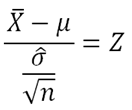
The method of solving this is just the same as method 1, but here we do not know the population variance. Using the unbiased estimate of population mean x̅ = μ, and the unbiased estimate of population variance,
Our confidence interval will be
or we could rewrite it in terms of s,
4. Non-normal with unknown variance σ2 (n ≥ 30)
Similar to method 2, we approximate a normal distribution, and after finding the sampling distribution X̅, we use the unbiased estimates μ̂ and σ̂, we use the same equation for confidence interval as the method 3,
5. Normal with unknown variance σ2 (n < 30)
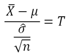
It is interesting to note that when the sample size is small, the sampling distribution
does not follow a normal distribution. Instead, it follows a t-distribution.
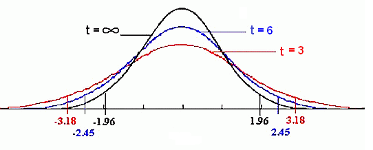
The distribution of T is a member of t-distributions. All t-distributions are symmetric about zero and have single parameter ν (pronouced ‘new’) which is a positive integer. ν is known as the number of degrees of freedom of the distribution and if, for example, T has a t-distribution with 5 degrees of freedom, you would write T ~ t(5). For a sample size n, it can be shown that T follows a t-distribution with (n – 1) degrees of freedom. Take a look at the t-distribution curves below.
Notice that we only use the t-distribution when the sample size is small, and therefore, when t tends to infinity, it will look like a normal curve. In other words, nothing much has changed, we are just using a new distribution for small sample size. After knowing that our sample size is small, we use the t-distribution using (n – 1) degrees of freedom, use the unbiased estimates for both the mean and the variance, and our new formula will be
where t can be obtained from the t-distribution tables. It looks something like this. The way you use it is exactly the same as the critical values for the normal distribution, its just that there is a column of degrees of freedom.
HOW TO SOLVE EXAM QUESTIONS
It isn’t hard. All you need to do is to identify the quantities stated in the question, and you’ll classify whether you should solve the question using which one of the 5 methods. I’ll put here a few example of questions, and show you how to analyse them:
A plant produces steel sheets whose weights are known to be normally distributed with a standard deviation of 2.4kg. A random sample of 36 sheets had a mean weight of 31.4kg. Find the 99% confidence interval for the population mean.
It is normally distributed, variance = 2.42kg (known), sample size = 36, sample mean = 31.4kg. Use method 1.
The heights of men in a particular district are distributed with mean μ cm and standard deviation σ cm. On the basis results obtained from a random sample of 100 men from the district the 95% confidence interval for μ was calculated and found to be (177.22cm, 179.18cm). Find the value of the σ and x̅.
Unknown distribution, variance known, but sample size large. Approximate normal, method 2. You need to work backwards using the confidence interval formulas, get 2 simultaneous equations, and solve for σ and x̅. Give it a try.
The fuel consumption of a new model of car is being tested. In one trial, 50 cars chosen at random, were driven under identical conditions and the distances, x km, covered on 1 litre of petrol were recorded. The results gave the following totals:
Σx = 525, Σx2 = 5625
Calculate a 95% confidence interval for the mean petrol consumption, in km/l, of cars of this type.
Unknown distribution, variance unknown, big sample. Approximate normal, use unbiased estimate of population variance (you have to calculate it this time), use method 4.
A sample of 8 independent observations of a normally distributed variable gave the following values: 3.6, 3.9, 4.5, 3.8, 4.4, 4.9, 4.2, 3.8. Determine a 99% confidence interval for the population mean μ.
Normal distribution, unknown variance, and small sample. Method 5. In your question, you need to write these sentences very clearly:
since n < 30, a t(n-1) distribution is used. T ~ t(7)
Then you continue to find the confidence intervals.
Not hard, isn’t it?
Here are a few short notes you might want to take note as well:
1. interval width
The width of a confidence interval can be obtained from the expression
Also remember, when the width is increased, then either
a. the sample size n increases,
b. the confidence interval decreases, or
c. the variance decreases.
2. Assumption
Many times you might be asked, “state the assumptions you made”. You probably only have one assumption, which is: we assume that it is a random sample.
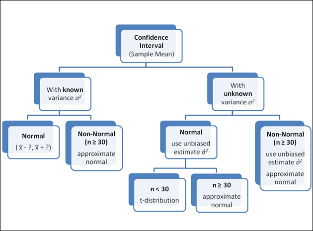
To summarize this section, I made a chart for you to remember things easier.
Take note that this is the most important section of this chapter. Be sure you are clear with all the distributions, don’t confuse the sample size n with the number of trials n in a Binomial distribution, and practise more on population proportions. ☺


No comments:
Post a Comment